
Lattice: an 8 MB static retriever that embeds Wikipedia in 7 minutes







- I trained
lattice-retrieval, a static embedding model, on 660M curated query/document pairs. It scores 0.4581 NDCG@10 on decontaminated BEIR before fine-tuning and 0.4749 after fine-tuning, compared with 0.4334 forsentence-transformers/static-retrieval-mrl-en-v1. - Static models are unusually forgiving quantization targets. The best quality/size trade-off I found is int4-row at 512 dimensions: a 7.94 MB weight file that scores 0.4697, effectively the same as fp32 at the same dimension.
- I built a pure-Rust runtime to embed all 6.4M articles in English Wikipedia in 7 minutes and 26 seconds on an 8-core Apple M2 MacBook Air.
Model
erikkaum/lattice-retrieval
· Code ErikKaum/lattice
What is a static embedding model?
A static embedding model embeds text with one learned lookup table followed by mean pooling. There is no attention, contextualization, or transformer stack. The forward pass is simply:
- Tokenize the text.
- Look up one vector per token.
- Average the vectors and L2-normalize the result.
For example, imagine that "hello world" tokenizes to [7592, 2088], and that
we have a tiny eight-dimensional embedding table. Looking up those two rows
might give us:
world [2088]:   [-0.020,  0.015, -0.036,  0.100,  0.000,  0.044, -0.051,  0.057 ]
...
hello [7592]:   [ 0.100,  0.000,  0.036, -0.100,  0.084,  0.000,  0.017, -0.038 ]
                ─────────────────────────────────────────────────────────────────
mean:           [ 0.040,  0.0075, 0.000,  0.000,  0.042,  0.022, -0.017,  0.0095]
The mean has a norm of about 0.06545, so after L2 normalization the final
embedding is:
[0.611, 0.115, 0.000, 0.000, 0.642, 0.336, -0.260, 0.145]
And that's the entire model. The same token always selects the same row; the surrounding words never change its vector.
That simplicity makes static models extremely fast and compact. It also gives them obvious limits: they do not model word order, polysemy, or compositional meaning nearly as well as a transformer. They're usually not used to build systems where the retriever quality has to be high.
But they're useful when throughput, cost, or deployment size matters more:
- hard-negative mining for training larger models;
- corpus-scale deduplication and clustering;
- first-stage candidate generation before a reranker;
- on-device and in-browser.
Models such as GloVe and
fastText established the basic idea at the word level
and more recent projects such as
model2vec / potion train static tables
specifically for sentence embeddings and retrieval, with their model potion-retrieval-32M scoring 0.512 on NanoBEIR. Similarly
static-retrieval-mrl-en-v1
is a top-performing model in this category
I wanted to find out how far we can push this simple architecture:
- Does it continue improving with substantially more curated data?
- Can hard-negative fine-tuning teach a bag-of-token-vectors model anything useful?
- How aggressively can the resulting table be quantized?
- How many tokens/sec can we achieve with a focused effort on improving the runtime performance?
This blog is my journey to answer the questions above. Enjoy!
Try it
The full-precision model follows the Sentence Transformers layout:
from sentence_transformers import SentenceTransformer

model = SentenceTransformer("erikkaum/lattice-retrieval")
embeddings = model.encode(
    ["hello world", "static embeddings are fast"],
    normalize_embeddings=True,
)
print(embeddings.shape)  # (2, 1024)
Generating a quantized artifact and running it in Rust have their own quickstart at the end of the article.
Part 1: Training with more, better-curated data
The reference point for this project is
sentence-transformers/static-retrieval-mrl-en-v1.
It's the exact same architecture and training objective, but trained from
scratch on a much larger corpus. The main enabler was
lightonai/embeddings-pre-training-curated:
665M query/document pairs curated from 34 sources, cross-encoder filtered with
mxbai-rerank-large-v2,
deduplicated.
I excluded three subsets with direct BEIR overlap, beir_dbpedia, msmarco,
and quora, leaving roughly 660M pairs. That is still about eight times the
training data used for the reference model.
I trained the model in two stages:
- Stage 1: contrastive pre-training on the 660M curated pairs.
- Stage 2: best-of-7 hard-negative fine-tuning on LightOn's
embeddings-fine-tuningrelease.
And as a reminder, the model architecture is simply a 30,522 by 1,024 matrix:
SentenceTransformer(
  (0): StaticEmbedding(
    (embedding): EmbeddingBag(30522, 1024, mode='mean')
  )
)
It uses the 30,522-token BERT-uncased vocabulary, mean pooling, and Matryoshka
training over dimensions [1024, 512, 256, 128, 64, 32]. The loss is
MultipleNegativesRankingLoss from Sentence Transformers. These are all the
same choices as in the static-retrieval-mrl-en-v1 model.
Making 660M pairs feed a tiny model fast
Static-model training is data-throughput-bound rather than compute-bound. A GPU can finish a batch almost immediately and then sit idle while Python reads parquet, tokenizes strings, pads examples, and collates the next batch. So to make the training as fast as possible, we have to think about our data access patterns and I/O. I ended up building a dataloader from scratch for this.
The core idea is to move as much work offline as possible. That is, to do work before the actual training run. The first obvious trick is to pre-tokenize the corpus. This runs on CPU and is easily parallelizable. After tokenization, I saved the data into flat binary files:
query_tokens.bin       query_offsets.bin
doc_tokens.bin         doc_offsets.bin
where the tokens are just one contiguous array and the offset binary contains
the row boundaries. So now to retrieve row i, the loader takes one slice:
tokens[offsets[i] : offsets[i + 1]]
As a concrete example, suppose we tokenize two queries:
query 0: "how do birds fly"       → [2129, 2079, 5055, 4875]
query 1: "when was rome founded"  → [2043, 2001, 4199, 2631]
They are laid out back-to-back in one token file, with a second file telling us where each row begins and ends:
query_offsets.bin (uint64)
    ┌─────┬─────┬─────┐
    │  0  │  4  │  8  │
    └──┬──┴──┬──┴──┬──┘
       │     │     │
       │     │     └───────────────────────────────────────────┐
       │     └─────────────────────┐                           │
       ▼                           ▼                           ▼
query_tokens.bin (uint16)
       ┌──────┬──────┬──────┬──────┬──────┬──────┬──────┬──────┐
       │ 2129 │ 2079 │ 5055 │ 4875 │ 2043 │ 2001 │ 4199 │ 2631 │
       └──────┴──────┴──────┴──────┴──────┴──────┴──────┴──────┘
         how    do    birds   fly    when   was   rome  founded
       └──────── query 0 ─────────┘└──────── query 1 ─────────┘
Reading query 1 is now simply query_tokens[4:8]. No parsing, decoding, or
extra allocations needed. At training time the files are memory-mapped as
contiguous batches, which allows the operating system's page cache to help keep
read latencies down. The document side uses exactly the same representation.
The corpus is also exposed through nested xs, small, medium, and full
tiers. A deterministic proportional schedule selects a prefix from each source,
so the tiers remain nested while approximately preserving the same mixture as
the full corpus. In short, xs ⊂ small ⊂ medium ⊂ full.
This access strategy relies on contiguous reads. If we jump from
query_tokens[4:8] to query_tokens[445:568] and so forth, we lose the
benefits the page cache gives us. But training still needs some shuffling. The
solution I went for was to have the training loader separately divide each
selected source prefix into contiguous batch_size windows, globally shuffle
those windows every epoch, and distribute them across the GPUs.
Each batch still comes from one source, so its in-batch negatives stay in-domain, while each disk read stays contiguous. So the trick is: shuffle batches for training quality, not individual rows at the cost of random I/O.
On four NVIDIA A100s, Stage 1 training sustained roughly 360–370K pairs/sec in aggregate. At that rate, one pass over 660M pairs is about 30 minutes of optimizer steps, excluding data staging, startup, checkpoints, and evaluation.
The implementation details, including tier planning and distributed batch partitioning, are in the pipeline and trainer directories.
Stage 1: data scaling works
The result is straightforward: this architecture continued improving as the corpus grew.
Stage-1 data scaling, NDCG@10 at 1024 dimensions
| Model | Training pairs | NanoBEIR | Decontaminated BEIR 12-mean |
|---|---|---|---|
static-retrieval-mrl-en-v1 |
~80M | 0.5032 | 0.4334 |
potion-retrieval-32M |
- | 0.512 | — |
| lattice xs | 10M | 0.4911 | — |
| lattice small | 100M | 0.5035 | — |
| lattice medium | 275M | 0.5143 | — |
| lattice full | 660M | 0.5212 | 0.4581 |
At 100M pairs, the model is essentially tied with the roughly 80M-pair reference. The 275M and 660M tiers move ahead, and the curve has not visibly flattened at the full tier. On decontaminated BEIR, the full Stage-1 model improves the 12-task mean by +0.0247.
Not a shocking result: eight times more curated data improved the model. But it establishes the baseline for the rest of the project.
The Matryoshka results across all four training tiers show how the extra data is distributed through the representation. All values below are NanoBEIR NDCG@10:
| Dimension | xs (10M) | small (100M) | medium (275M) | full (660M) | Reference |
|---|---|---|---|---|---|
| 1024 | 0.4911 | 0.5035 | 0.5143 | 0.5212 | 0.5032 |
| 512 | 0.4872 | 0.5036 | 0.5113 | 0.5201 | — |
| 256 | 0.4808 | 0.4978 | 0.5017 | 0.5135 | — |
| 128 | 0.4526 | 0.4719 | 0.4732 | 0.4899 | — |
| 64 | 0.4087 | 0.4243 | 0.4283 | 0.4406 | — |
| 32 | 0.3420 | 0.3596 | 0.3554 | 0.3624 | — |
The scaling isn't uniform. Between 100M and 275M pairs, the gain is +0.0108 at 1024 dimensions and +0.0077 at 512, compared with +0.0013 at 128 and a slight regression at 32. The full tier lifts almost every width again. Wider subspaces benefit more consistently, while the smallest dimensions appear noisier and closer to their capacity. This is consistent with ZeroEntropy's argument that Matryoshka concentrates information into its leading dimensions at a cost to the rest of the representation. A task-specific learned projection might recover quality that simple truncation leaves on the table.
Stage 2: hard negatives help, modestly
Honestly, I didn't expect hard negative fine-tuning to give the model a big uplift. It has no attention mechanism for the fine distinctions that hard negatives are usually intended to teach. But with the training infra already set up and ready to go, why not satisfy my curiosity: can a mean-pooled lookup table learn from hard negatives at all?
Starting from the full Stage-1 checkpoint, I fine-tuned for 10 epochs on
LightOn's seven-source
lightonai/embeddings-fine-tuning
dataset. For each pair I retained the top 50 mined negatives scoring below 0.95
times the query-positive similarity, discarded examples without enough eligible
negatives, and sampled seven negatives during training.
The filter removed 17% of pairs, concentrated in TriviaQA and NQ. Many of their high-scoring mined “negatives” are likely alternate correct answers, which is exactly what the similarity cutoff is intended to catch.
Stage-2 lift over Stage 1, NDCG@10 at 1024 dimensions
| Evaluation | Stage 1 | Stage 2 | Change |
|---|---|---|---|
| Held-out in-domain | 0.8107 | 0.8359 | +0.0252 |
| Decontaminated BEIR 12-mean | 0.4581 | 0.4749 | +0.0168 |
| Decontaminated BEIR 5-task diagnostic | 0.4537 | 0.4684 | +0.0147 |
The five-task diagnostic is the unweighted mean over ArguAna, Touché2020, Quora, ClimateFEVER, and TREC-COVID. I treat it as a directional slice rather than a headline metric because several of those decontaminated tasks retain very few scored queries.
The static model does learn from hard negatives. The same recipe family improved DenseOn by +0.0715 on BEIR in LightOn's DenseOn/LateOn article; lattice gets +0.0168 on the decontaminated 12-task mean. This is only a directional comparison, not a controlled head-to-head, but the smaller gain is approximately what we expected from this architecture. Since the fine-tuning data overlaps heavily with standard BEIR and NanoBEIR tasks, I don't use the absolute Stage-2 NanoBEIR score as evidence of generalization. The evaluation appendix explains the held-out and decontaminated surfaces in more detail.
Part 2: Quantization
Remember that the model is just a single [30,522, 1,024] floating-point
matrix. The beauty is that the simplicity of the model makes it less capable
than transformer-based ones, but these same limitations also make it an
unusually clean target for post-training quantization:
- quantization error is introduced once, rather than repeatedly across a deep network;
- there are no intermediate activations to quantize;
- mean pooling can suppress some weakly correlated token-level error;
- final L2 normalization removes uniform positive rescaling, though not direction-changing error.
I went for a symmetric weight-only quantization at several bit widths and Matryoshka dimensions. In symmetric quantization, a group of floating-point weights shares a scale:
qmax  = 2^(bits - 1) - 1
scale = max(abs(weights in group)) / qmax
q     = round(weight / scale)
w̃     = q × scale
So int8 represents weights with integer codes from -127 to +127, int4 uses
-7 to +7, and int2 uses only -1, 0, and +1. The scale stretches that
small integer grid across the floating-point range of the group. At int8 the
grid is dense enough to look almost continuous; at int2 every weight must become
negative, zero, or positive at exactly one magnitude.
Let's do a quick concrete example using this tiny four-token, six-dimensional embedding table:
                   d0     d1     d2     d3     d4     d5      max|w| in row
                ┌───────────────────────────────────────────┐
        token 0 │ 0.92  -0.31   0.12  -0.05   0.44  -0.78   │     0.92
        token 1 │ 0.08  -0.11   0.06  -0.09   0.05  -0.07   │     0.11
        token 2 │-0.55   0.61  -0.48   0.50  -0.52   0.58   │     0.61
        token 3 │ 0.21  -0.19   0.88  -0.22   0.18  -0.20   │     0.88
                └───────────────────────────────────────────┘
max|w| in col:    0.92   0.61   0.88   0.50   0.52   0.78
Let's quantize token 0 to int8 along the row. We obtain the scale by taking
0.92/127 = 0.00724, 127 being qmax for int8. Then, to obtain the individual
weights, we simply divide each weight by the scale and round.
Thus token 0 becomes:
token 0 codes: [ 127, -43, 17, -7, 61, -108 ]
Conceptually, inference reconstructs fp32 values rather than multiplying int8 weights directly. The storage and bandwidth gain comes from moving the int8 codes. Later we'll see how the runtime avoids materializing these reconstructed rows by accumulating the integer codes first. We can check the floating-point reconstruction by multiplying the scale with the codes:
w̃: [ 0.920, -0.311, 0.123, -0.051, 0.442, -0.782 ]
And you can see that the reconstructed values are very close to the original ones: the max error is just 0.003. The next design choice is whether the group comes from quantizing along the dimension or row axis.
Note: quantization happens after Matryoshka slicing. When I evaluate at, say, dim=256, I slice the table to its first 256 columns and then compute scales on the slice. Each Matryoshka dimension is therefore its own quantized model with its own scales, rather than a truncation of the 1024-dim scales.
Per-row or per-dim scaling?
With per-dim quantization, each embedding-table column gets one scale. This is convenient at inference time: token rows can be accumulated as integers and each output dimension is scaled once at the end.
With per-row quantization, each token gets its own scale. The runtime is slightly more involved, but every token receives a quantization grid matched to its own magnitude.
Using the same toy example, let's look at token 1 now:
                   d0     d1     d2     d3     d4     d5      max|w| in row
                ┌───────────────────────────────────────────┐
        token 0 │ 0.92  -0.31   0.12  -0.05   0.44  -0.78   │     0.92
        token 1 │ 0.08  -0.11   0.06  -0.09   0.05  -0.07   │     0.11
        token 2 │-0.55   0.61  -0.48   0.50  -0.52   0.58   │     0.61
        token 3 │ 0.21  -0.19   0.88  -0.22   0.18  -0.20   │     0.88
                └───────────────────────────────────────────┘
max|w| in col:    0.92   0.61   0.88   0.50   0.52   0.78
Token 1 is much "quieter" than the other tokens: its largest magnitude is only
0.11, which can become an issue if we scale per-dim. Let's illustrate this by
looking at what int2 per-row and per-dim quantization does to this token.
With int2 per-row quantization, it gets its own 0.11 scale and remains
nonzero:
token 1 original:  [ 0.08, -0.11,  0.06, -0.09,  0.05, -0.07 ]
int2 per-row code: [    1,    -1,     1,    -1,     0,    -1 ]
With per-dim quantization, the scale in each column is set by a much louder token. At int2, every value in token 1 rounds to zero:
int2 per-dim code: [ 0, 0, 0, 0, 0, 0 ]
So per-dim quantization has erased that token completely. Per-row scaling adapts to the dynamic range between tokens; per-dim scaling has to absorb it. The difference matters because token-row magnitudes vary far more than dimension magnitudes in the trained model. These statistics come directly from the final Stage-2 weights:
| Statistic | Token rows | Dimensions |
|---|---|---|
| Max-absolute dynamic range | 97.8× | 3.7× |
| L2-norm dynamic range | 56.9× | 2.3× |
At low bit widths, a quiet token quantized against a much louder column can disappear completely. Counting all-zero token rows after per-dim quantization makes the failure mode visible:
| Bit width | All-zero token rows |
|---|---|
| int8 | 2 (0.01%) |
| int4 | 1,432 (4.69%) |
| int3 | 1,666 (5.46%) |
| int2 | 7,715 (25.28%) |
The two rows that remain zero even at int8 are [CLS] and [SEP].
StaticEmbedding tokenizes with add_special_tokens=False, so neither token
participates in the mean-pooled embedding and their rows are deliberately kept
at zero. In other words, int8 introduces no new silent tokens. Per-row
quantization also creates no additional silent rows because every nonzero row's
largest value reaches the edge of its own grid.
Why is the dynamic range so asymmetric? A row belongs to one token, and nothing requires every token to contribute at the same magnitude. A dimension, on the other hand, is measured across all 30,522 tokens: even if most entries in a column are small, there are thousands of opportunities for some token to have a large value there, and its L2 norm aggregates the whole vocabulary. Matryoshka training may contribute too, since the leading dimensions participate in more truncated objectives.
Note that this does not mean per-row is always better. At int8 there is essentially no quality difference, while per-dim scaling enables a simpler and faster integer kernel. The axis only becomes important at the lower bit widths.
Quantization results
The toy example tells us why the scaling axis might matter, but the final question is empirical: how much retrieval quality survives when we reduce precision and dimension? I swept the complete variant matrix on NanoBEIR, then reran the promising deployment artifacts on the full decontaminated BEIR evaluation.
| Variant | Weight file | Decontaminated BEIR 12-mean | Change from same-dim fp32 |
|---|---|---|---|
| fp32-dim-1024 | 125.02 MB | 0.4749 | — |
| int8-dim-1024 | 31.26 MB | 0.4747 | −0.0002 |
| fp32-dim-512 | 62.51 MB | 0.4697 | — |
| int4-row-512 | 7.94 MB | 0.4697 | −0.0001 |
| int4-dim-512 | 7.82 MB | 0.4629 | −0.0068 |
| int2-row-1024 | 7.94 MB | 0.4185 | −0.0564 |
Int8 is practically lossless. At 512 dimensions, int4-row is almost eight times smaller than fp32 and has the same quality to four decimal places. Int4-dim loses 0.0068, partly because its shared column scales silence some quiet tokens. Int2-row avoids that failure mode, but its ternary grid is simply too coarse and loses 0.0564.
Part 3: Fast inference on CPU
The final part is making these models fast on consumer hardware. One of the main appeals of this architecture is that we should be able to process a lot of text fast and cheaply. I built a pure-Rust runtime for the truncated and quantized models. It memory-maps the model weights, uses SIMD kernels, parallelizes over input chunks, and streams fp32 embeddings to disk.
The most important trick is that we don't need to dequantize every token row
before calculating the mean. In the int4 model, two codes fit in each byte. The
conceptual signed codes from -7 to +7 are physically stored as unsigned
values from 0 to 14, biased by +7. With per-dim scales, an individual
weight is reconstructed as:
weight[token, d] ≈ (code[token, d] - 7) × scale[d]
Now let's reuse the "hello world" example from the beginning. The two packed
rows unpack to these codes:
hello codes: [12,  7,  9,  3, 14,  7,  8,  5]
world codes: [ 6,  8,  5, 11,  7,  9,  4, 10]
scale[d]:    [.020, .015, .018, .025, .012, .022, .017, .019]
We could subtract 7, multiply by the scale, and produce a temporary fp32 row
for every token. But because scale[d] is shared by all tokens, we can move it
outside the sum:
mean[d] = scale[d] / N × (Σ code[token, d] - 7N)
So the hot loop only unpacks and adds integers:
hello codes:  [12,  7,  9,  3, 14,  7,  8,  5]
world codes:  [ 6,  8,  5, 11,  7,  9,  4, 10]
               ─────────────────────────────────
integer sum:  [18, 15, 14, 14, 21, 16, 12, 15]

subtract 7N: [ 4,  1,  0,  0,  7,  2, -2,  1]
× scale / N: [.040, .0075, 0, 0, .042, .022, -.017, .0095]
That final line is the same mean vector we calculated from fp32 weights at the beginning of the article. We get there without ever materializing the dequantized rows: accumulate the packed integer codes first, then fuse bias correction, scaling, and averaging into one final pass before L2 normalization.
This also explains why per-dim quantization gives us a nicer inference kernel than per-row quantization. With one scale per row, the equation becomes:
mean[d] = 1 / N × Σ scale[token] × (code[token, d] - 7)
The scale changes for every token, so it cannot be moved outside the sum. The per-row kernel still fuses unpacking, scaling, and accumulation. It does not build a dequantized table either, but it has to perform floating-point multiply-adds inside the token loop. The per-dim kernel gets away with integer additions and one scale application per output dimension at the end.
Note that smaller bit widths do not guarantee more speed. Int2 moves fewer bytes, but unpacking four sub-byte values costs more instructions. Int8 is larger but native. The best representation depends on memory bandwidth, vectorization, dimension, and scale layout, so it has to be measured rather than inferred from file size.
This is the trade-off we saw in the previous section. Per-dim scaling gives us the cleaner kernel, but a shared column scale can erase quiet tokens at very low precision. Per-row scaling protects those tokens at the cost of more work in the hot loop. At int4-512, the end-to-end difference is marginal: 9.03M tokens/sec for per-dim versus 8.76M for per-row because tokenization dominates the full pipeline.
Quality and throughput across the full variant matrix
Putting the quality and runtime measurements together gives us the full set of operating points:
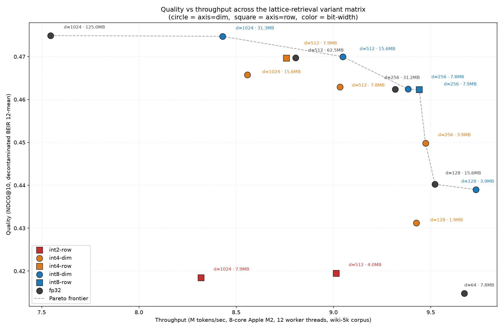
Every point is one run over the same 5,000-article corpus with 12 worker threads
on the same 8-core Apple M2 MacBook Air. The Pareto frontier marks variants for
which there is no measured alternative that is both faster and better. At the
quality-first end, fp32-1024 is best, but int8-dim-1024 gets essentially the
same quality with one quarter of the weight storage. The measurements are
intended to show the operating-point trade-offs, not to be a cross-machine CPU
benchmark. The underlying numbers are available in
data/quality_vs_throughput.csv.
Benchmark: English Wikipedia
To have a somewhat realistic workload to benchmark on, I flattened the
wikimedia/wikipedia 20231101.en snapshot
to one article per line and embedded all 6,407,814 articles with the
int4-dim-512 artifact.
On an 8-core Apple M2 MacBook Air with 12 worker threads, the run took:
7 minutes and 26 seconds — 9.52M tokens/sec, or about 14,400 articles/sec.
The phase breakdown was:
| Phase | Share of runtime |
|---|---|
| Tokenization | 91.7% |
| Model lookup, accumulation, and normalization | 6.1% |
| Writing output | 0.4% |
| Orchestration overhead | 1.8% |
We've reached the point where the model itself is just a fraction of the end-to-end latency, and tokenization is now the bottleneck. Nice!
Summary
We've touched a lot of things here: starting from a simple data scaling question and going through data layout, training infrastructure, evaluation contamination, quantization geometry, binary formats, and inference.
The takeaways map directly back to the questions I started with:
- More curated data still helps. Stage 1 kept improving through the full 660M-pair tier.
- Hard negatives can teach a static model, modestly. Stage 2 added +0.0168 on the decontaminated BEIR mean. Useful, but much less than the +0.0715 DenseOn result.
- Static embedding models quantize extremely well. Int8 was nearly free, and the scaling axis matters once precision gets low.
- A focused runtime makes corpus-scale embedding a laptop job. The final pipeline reached 9.52M tokens/sec, with tokenization accounting for 91.7% of the runtime.
Maybe as a final note: the resulting system is not a replacement for a strong transformer retriever. It is a compact, extremely fast first-stage model that can be shipped almost anywhere, used to mine or cluster enormous corpora, and run cheaply enough that embedding all of English Wikipedia becomes a laptop-scale job.
Use it for what it's good for.
Appendix: Stage-2 evaluation details
The Stage-2 dataset contains FiQA, NQ, HotpotQA, MS MARCO, FEVER, SQuAD v2, and TriviaQA. Its overlap with BEIR means the fine-tuned model's absolute NanoBEIR score is contaminated. So I use Stage-2 NanoBEIR only for paired post-training-quantization comparisons against the fp32 checkpoint.
The main reported surfaces are:
- a seed-fixed, query-level held-out set from the seven fine-tuning sources, used to measure in-domain lift;
- LightOn's decontaminated BEIR suite, used as the noisier generalization check.
The decontaminated suite removes corpus documents matching the fine-tuning data and then removes queries that lose all relevant documents. This avoids direct document overlap, but some tasks are left with much smaller candidate pools or very few scored queries. For example, NQ retains 26 scored queries and MSMARCO 41. The aggregate is useful for model-to-model comparison, but it is not the original BEIR distribution restored to a pristine state.
The 12-task values are unweighted means following LightOn's convention of excluding ClimateFEVER and FEVER. I also computed the 14-task mean for completeness:
| Dimension | Reference 12 | Stage 1 12 | Stage 2 12 | Stage 2 14 |
|---|---|---|---|---|
| 1024 | 0.4334 | 0.4581 | 0.4749 | 0.4581 |
| 512 | 0.4297 | 0.4540 | 0.4697 | 0.4527 |
| 256 | 0.4213 | 0.4444 | 0.4624 | 0.4438 |
| 128 | 0.4101 | 0.4270 | 0.4402 | 0.4205 |
| 64 | 0.3663 | 0.3971 | 0.4148 | 0.3902 |
| 32 | 0.2991 | 0.3325 | 0.3262 | 0.3013 |
The canonical fp32
per-task results and corpus-removal statistics
and the corresponding JSONs for all deployment variants are checked in under
data/. The
repository evaluation notes
summarize the comparisons and document the evaluation commands.
Reproducibility and artifacts
The repository includes a slicer/quantizer and a pure-Rust runtime. The canonical fp32 model lives on Hugging Face and deployment variants are generated locally rather than published as dozens of separate artifacts.
Rust CLI
First use the slicer tool to generate the desired quantization & truncation
combination:
git clone https://github.com/ErikKaum/lattice
cd lattice/slicer
uv run slicer slice \
  --dim 512 \
  --quant int4_dim \
  --output-dir ../data/int4-dim-512
And then the Rust runtime to generate the embeddings:
cd ../lattice
cargo build --release --bin embed

echo "hello world" \
  | ./target/release/embed \
      --model ../data/int4-dim-512/model.safetensors \
      --output /tmp/embedding.bin
The output is a flat fp32 matrix, ready to load into an ANN index or another application.
Python bindings
For convenience, the Rust runtime also comes with Python bindings. You can build them using maturin:
# From the repository root:
cd lattice
uv venv .venv-py
source .venv-py/bin/activate
uv pip install maturin numpy
maturin develop --release --features python
import numpy as np
import lattice

model = lattice.Model.load("../data/int4-dim-512/model.safetensors")
tokenizer = lattice.Tokenizer.load("../data/int4-dim-512/tokenizer.json")

texts = ["hello world", "static embeddings are fast"]
token_ids = tokenizer.encode_batch(texts)
embeddings = np.stack([
    model.embed(ids, normalize=True)
    for ids in token_ids
])

print(model.variant, model.dim)  # int4_dim 512
print(embeddings.shape)          # (2, 512)
The bindings call the same Rust tokenizer and embedding kernels as the command-line runtime. They just return NumPy arrays instead of writing a flat binary file.
Artifact links
- Full-precision model
- Training, quantization, and evaluation code
- Pre-tokenization and mmap pipeline
- Slicing and quantization tool
- Pure-Rust runtime
- Decontaminated-BEIR harness
- Benchmark and quality data
Acknowledgements
The data, fine-tuning recipe, and decontaminated evaluation splits are LightOn's
(DenseOn/LateOn); this
work is a static-model study built on their release. The reference architecture
and static-embedding training recipe are from the Sentence Transformers team's
static-retrieval-mrl-en-v1.
The Matryoshka discussion draws on
ZeroEntropy and
related
work.


